The t distribution is used to form confidence limits and perform statistical tests to answer the question that a variable in a study group is significantly different from a norm or population mean?
How?
Example
If the mean of a variable is much larger or smaller than the mean in the norm such as the situation in Figure Belwo, we will probably conclude that the difference is real.
Comparison of distributions.
++What other factors can help us? Figure 5–1B gives a clue: The sample values vary substantially, compared with Figure 5–1A, in which there is less variation. A smaller standard deviation may lead to a real difference, even though the difference is relatively small. For the variability to be small, subjects must be relatively similar (homogeneous) and the method of measurement must be relatively precise. In contrast, if the characteristic measured varies widely from one person to another or if the measuring device is relatively crude, the standard deviations will be greater, and we will need to observe a greater difference to be convinced that the difference is real and not just a random occurrence.
++Another factor is the number of patients included in the sample. Most of us have greater intuitive confidence in findings that are based on a larger rather than a smaller sample, and we will demonstrate the sound statistical reasons for this confidence.
To summarize, three factors play a role in deciding whether an observed mean differs from a norm: (1) the difference between the observed mean and the norm, (2) the amount of variability among subjects, and (3) the number of subjects in the study. We will see later in this chapter that the first two factors are important when we want to estimate the needed sample size before beginning a study.
Adjustment: To adjust for the influence of confounding variables and interactions on the estimates and inferences.
Is there a difference in means or medians (ordinal or numerical measures)?
Is there a difference in means or medians (ordinal or numerical measures)?can express ed the difference ]
+++++++++++++
Confidence interval=Mean difference±Number related to confidence level (often 95% ) × Standard error of the differenceConfidence interval=Mean difference±Number related to confidence level (often 95%) × Standard error of the differenceIf we use symbols to illustrate a confidence interval for the difference between two means and let X ¯ ¯ ¯ 1X¯1 stand for the mean of the first group and X ¯ ¯ ¯ 2X¯2 for the mean of the second group, then we can write the difference between the two means as X ¯ ¯ ¯ 1−X ¯ ¯ ¯ 2X¯1−X¯2.
As you know from the previous chapter, the number related to the level of confidence is the critical value from the t distribution. For two means, we use the t distribution with (n1 − 1) degrees of freedom corresponding to the number of subjects in group 1, plus (n2 − 1) degrees of freedom corresponding to the number of subjects in group 2, for a total of (n1 + n2 − 2) degrees of freedom.
+++++++++++++
The t Distribution and Confidence Intervals About the Mean in One Group
Confidence intervals are used increasingly for research involving means, proportions, and other statistics in medicine, and we will encounter them in subsequent chapters. Thus, it is important to understand the basics. The general format for confidence intervals for one mean is:
Observed mean±(Confidence coefficient) × (A measure of variability of the mean)
+++++++++++++++++++++++++++++
t test
The t -test is used to determine with some degree of confidence that the difference might have occurred by chance or is actual between groups.
The t test tells how significant the differences between groups are.By inference, the same difference also exists in the population from which the sample was drawn.
We assume the dependent variable fits a normal distribution.
When we assume a normal distribution exists, we can identify the probability of a particular outcome.
The test statistic that a t test produces is a t-value.
Conceptually, t-values are an extension of z-scores.
In a way, the t-value represents how many standard units the means of the two groups are apart.
t-test calculation example
t test compares the mean of your sample data to a known value.
For example, you might want to know how your sample mean compares to the population mean. You should run a one sample t test when you don’t know the population standard deviation or you have a small sample size. For a full rundown on which test to use, see: T-score vs. Z-Score.
Assumptions of the test (your data should meet these requirements for the test to be valid):
- Data is independent.
- Data is collected randomly.
- The data is approximately normally distributed.
One Sample T Test Example
Sample question: your company wants to improve sales. Past sales data indicate that the average sale was $100 per transaction. After training your sales force, recent sales data (taken from a sample of 25 salesmen) indicates an average sale of $130, with a standard deviation of $15. Did the training work? Test your hypothesis at a 5% alpha level.
Step 1: Write your null hypothesis statement (How to state a null hypothesis). The accepted hypothesis is that there is no difference in sales, so:
H0: μ = $100.Step 2: Write your alternate hypothesis. This is the one you’re testing. You think that there is a difference (that the mean sales increased), so:
H1: μ > $100.Step 3: Identify the following pieces of information you’ll need to calculate the test statistic. The question should give you these items:
- The sample mean(x̄). This is given in the question as $130.
- The population mean(μ). Given as $100 (from past data).
- The sample standard deviation(s) = $15.
- Number of observations(n) = 25.
Step 4: Insert the items from above into the t score formula.
t = (130 – 100) / ((15 / √(25))
t = (30 / 3) = 10
This is your calculated t-value.Step 5: Find the t-table value. You need two values to find this:
- The alpha level: given as 5% in the question.
- The degrees of freedom, which is the number of items in the sample (n) minus 1: 25 – 1 = 24.
Look up 24 degrees of freedom in the left column and 0.05 in the top row. The intersection is 1.711.This is your one-tailed critical t-value.
What this critical value means is that we would expect most values to fall under 1.711. If our calculated t-value (from Step 4) falls within this range, the null hypothesis is likely true.
Step 5: Compare Step 4 to Step 5. The value from Step 4 does not fall into the range calculated in Step 5, so we can reject the null hypothesis. The value of 10 falls into the rejection region (the left tail).
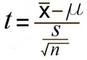
The formula for the t test has the observed mean minus the hypothesized value of the population mean (μ) in the numerator, and the standard error of the mean in the denominator. The symbol μ stands for the true mean in the population; it is the Greek letter mu, pronounced “mew.” The formula for the t test is
[Need Calculator]
References
1. https://www.statisticshowto.com/probability-and-statistics/t-test/
2. https://www.socscistatistics.com/tests/studentttest/default.aspx
3. http://www.sthda.com/english/wiki/t-test-formula
+++++++++++++++
Example: Let’s say you have a cold and you try a naturopathic remedy. Your cold lasts a couple of days. The next time you have a cold, you buy an over-the-counter pharmaceutical and the cold lasts a week. You survey your friends and they all tell you that their colds were of a shorter duration (an average of 3 days) when they took the homeopathic remedy. What you really want to know is, are these results repeatable? A t test can tell you by comparing the means of the two groups and letting you know the probability of those results happening by chance
If the t test produces a t-value that results in a probability of .01, we say that the likelihood of getting the difference we found by chance would be 1 in a 100 times. We could say that it is unlikely that our results occurred by chance and the difference we found in the samples probably exists between the groups from which the samples were was drawn.
FIVE FACTORS CONTRIBUTE TO WHETHER THE DIFFERENCE BETWEEN TWO GROUPS’ MEANS CAN BE CONSIDERED SIGNIFICANT:
- How large is the difference between the means of the two groups? Other factors being equal, the greater the difference between the two means, the greater the likelihood that a statistically significant mean difference exists. If the means of the two groups are far apart, we can be fairly confident that there is a real difference between them.
- How much overlap is there between the groups? This is a function of the variation within the groups. Other factors being equal, the smaller the variances of the two groups under consideration, the greater the likelihood that a statistically significant mean difference exists. We can be more confident that two groups differ when the scores within each group are close together.
- How many subjects are in the two samples? The size of the sample is extremely important in determining the significance of the difference between means. With increased sample size, means tend to become more stable representations of group performance. If the difference we find remains constant as we collect more and more data, we become more confident that we can trust the difference we are finding.
- What alpha level is being used to test the mean difference (how confident do you want to be about your statement that there is a mean difference). A larger alpha level requires less difference between the means. It is much harder to find differences between groups when you are only willing to have your results occur by chance 1 out of a 100 times (p < .01) as compared to 5 out of 100 times (p < .05).
- Is a directional (one-tailed) or non-directional (two-tailed) hypothesis being tested? Other factors being equal, smaller mean differences result in statistical significance with a directional hypothesis. For our purposes we will use non-directional (two-tailed) hypotheses.
+++++++++++++++
We specify the level of probability (alpha level, level of significance, p) we are willing to accept before we collect data (p < .05 is a common value that is used).
After we collect data we calculate a test statistic with a formula. We compare our test statistic with a critical value found on a table to see if our results fall within the acceptable level of probability.
[Modern computer programs calculate the test statistic for us and also provide the exact probability of obtaining that test statistic with the number of subjects we have.}
(the means must be measured on an interval or ratio measurement scale).Example
[Compare the reading achievement of boys and girls. With a t test, we have one independent variable and one dependent variable. The independent variable (gender in this case) can only have two levels (male and female). The dependent variable would be reading achievement.
If the independent had more than two levels, then we would use a one-way analysis of variance (ANOVA).
The test statistic that a t test produces is a t-value. Conceptually, t-values are an extension of z-scores. In a way, the t-value represents how many standard units the means of the two groups are apart.
With a t test, the researcher wants to state with some degree of confidence that the obtained difference between the means of the sample groups is too great to be a chance event and that some difference also exists in the population from which the sample was drawn. In other words, the difference that we might find between the boys’ and girls’ reading achievement in our sample might have occurred by chance, or it might exist in the population. If our t test produces a t-value that results in a probability of .01, we say that the likelihood of getting the difference we found by chance would be 1 in a 100 times. We could say that it is unlikely that our results occurred by chance and the difference we found in the sample probably exists in the populations from which it was drawn.
+++++++++++++
The t distribution is used to form confidence limits and perform statistical tests to answer the question that a variable in a study group is significantly different from a norm or population mean?
How?
Example
If the mean of a variable is much larger or smaller than the mean in the norm such as the situation in Figure Belwo, we will probably conclude that the difference is real.
Comparison of distributions.
++What other factors can help us? Figure 5–1B gives a clue: The sample values vary substantially, compared with Figure 5–1A, in which there is less variation. A smaller standard deviation may lead to a real difference, even though the difference is relatively small. For the variability to be small, subjects must be relatively similar (homogeneous) and the method of measurement must be relatively precise. In contrast, if the characteristic measured varies widely from one person to another or if the measuring device is relatively crude, the standard deviations will be greater, and we will need to observe a greater difference to be convinced that the difference is real and not just a random occurrence.
++Another factor is the number of patients included in the sample. Most of us have greater intuitive confidence in findings that are based on a larger rather than a smaller sample, and we will demonstrate the sound statistical reasons for this confidence.
To summarize, three factors play a role in deciding whether an observed mean differs from a norm: (1) the difference between the observed mean and the norm, (2) the amount of variability among subjects, and (3) the number of subjects in the study. We will see later in this chapter that the first two factors are important when we want to estimate the needed sample size before beginning a study.
Adjustment: To adjust for the influence of confounding variables and interactions on the estimates and inferences.
Is there a difference in means or medians (ordinal or numerical measures)?can express ed the difference ]
+++++++++++++
Confidence interval=Mean difference±Number related to confidence level (often 95% ) × Standard error of the differenceConfidence interval=Mean difference±Number related to confidence level (often 95%) × Standard error of the differenceIf we use symbols to illustrate a confidence interval for the difference between two means and let X ¯ ¯ ¯ 1X¯1 stand for the mean of the first group and X ¯ ¯ ¯ 2X¯2 for the mean of the second group, then we can write the difference between the two means as X ¯ ¯ ¯ 1−X ¯ ¯ ¯ 2X¯1−X¯2.
As you know from the previous chapter, the number related to the level of confidence is the critical value from the t distribution. For two means, we use the t distribution with (n1 − 1) degrees of freedom corresponding to the number of subjects in group 1, plus (n2 − 1) degrees of freedom corresponding to the number of subjects in group 2, for a total of (n1 + n2 − 2) degrees of freedom.
+++++++++++++
The t Distribution and Confidence Intervals About the Mean in One Group
Observed mean±(Confidence coefficient) × (A measure of variability of the mean)
++++++++++++++++++++++++++++++
The t test tells how significant the differences between groups are.
By inference, the same difference also exists in the population from which the sample was drawn.
We assume the dependent variable fits a normal distribution.
When we assume a normal distribution exists, we can identify the probability of a particular outcome.
The test statistic that a t test produces is a t-value. Conceptually, t-values are an extension of z-scores. In a way, the t-value represents how many standard units the means of the two groups are apart.+++++++++++++++++++++++
> Next: Variable Expressed by Proportions
Are Two Separate or Independent Groups Different
When the Variable Expressed by Means?
t test
t test compares the mean of your sample data to a known value. For example, you might want to know how your sample mean compares to the population mean.
[You should run a one sample t test when you don’t know the population standard deviation or you have a small sample size. For a full rundown on which test to use, see: T-score vs. Z-Score.
t-test calculation example
Assumptions of the test (your data should meet these requirements for the test to be valid):
- Data is independent.
- Data is collected randomly.
- The data is approximately normally distributed.
One Sample T Test Example
Sample question: your company wants to improve sales. Past sales data indicate that the average sale was $100 per transaction. After training your sales force, recent sales data (taken from a sample of 25 salesmen) indicates an average sale of $130, with a standard deviation of $15. Did the training work? Test your hypothesis at a 5% alpha level.
Step 1: Write your null hypothesis statement (How to state a null hypothesis). The accepted hypothesis is that there is no difference in sales, so:
H0: μ = $100.
Step 2: Write your alternate hypothesis. This is the one you’re testing. You think that there is a difference (that the mean sales increased), so:
H1: μ > $100.
Step 3: Identify the following pieces of information you’ll need to calculate the test statistic. The question should give you these items:
- The sample mean(x̄). This is given in the question as $130.
- The population mean(μ). Given as $100 (from past data).
- The sample standard deviation(s) = $15.
- Number of observations(n) = 25.
Step 4: Insert the items from above into the t score formula.
t = (130 – 100) / ((15 / √(25))
t = (30 / 3) = 10
This is your calculated t-value.
Step 5: Find the t-table value. You need two values to find this:
- The alpha level: given as 5% in the question.
- The degrees of freedom, which is the number of items in the sample (n) minus 1: 25 – 1 = 24.
Look up 24 degrees of freedom in the left column and 0.05 in the top row. The intersection is 1.711.This is your one-tailed critical t-value.
What this critical value means is that we would expect most values to fall under 1.711. If our calculated t-value (from Step 4) falls within this range, the null hypothesis is likely true.
Step 5: Compare Step 4 to Step 5. The value from Step 4 does not fall into the range calculated in Step 5, so we can reject the null hypothesis. The value of 10 falls into the rejection region (the left tail).
The formula for the t test has the observed mean minus the hypothesized value of the population mean (μ) in the numerator, and the standard error of the mean in the denominator. The symbol μ stands for the true mean in the population; it is the Greek letter mu, pronounced “mew.” The formula for the t test is

References
1. https://www.statisticshowto.com/probability-and-statistics/t-test/
2. https://www.socscistatistics.com/tests/studentttest/default.aspx
3. http://www.sthda.com/english/wiki/t-test-formula
+++++++++++++++
Example: Let’s say you have a cold and you try a naturopathic remedy. Your cold lasts a couple of days. The next time you have a cold, you buy an over-the-counter pharmaceutical and the cold lasts a week. You survey your friends and they all tell you that their colds were of a shorter duration (an average of 3 days) when they took the homeopathic remedy. What you really want to know is, are these results repeatable? A t test can tell you by comparing the means of the two groups and letting you know the probability of those results happening by chance
If the t test produces a t-value that results in a probability of .01, we say that the likelihood of getting the difference we found by chance would be 1 in a 100 times. We could say that it is unlikely that our results occurred by chance and the difference we found in the samples probably exists between the groups from which the samples were was drawn.
FIVE FACTORS CONTRIBUTE TO WHETHER THE DIFFERENCE BETWEEN TWO GROUPS’ MEANS CAN BE CONSIDERED SIGNIFICANT:
- How large is the difference between the means of the two groups? Other factors being equal, the greater the difference between the two means, the greater the likelihood that a statistically significant mean difference exists. If the means of the two groups are far apart, we can be fairly confident that there is a real difference between them.
- How much overlap is there between the groups? This is a function of the variation within the groups. Other factors being equal, the smaller the variances of the two groups under consideration, the greater the likelihood that a statistically significant mean difference exists. We can be more confident that two groups differ when the scores within each group are close together.
- How many subjects are in the two samples? The size of the sample is extremely important in determining the significance of the difference between means. With increased sample size, means tend to become more stable representations of group performance. If the difference we find remains constant as we collect more and more data, we become more confident that we can trust the difference we are finding.
- What alpha level is being used to test the mean difference (how confident do you want to be about your statement that there is a mean difference). A larger alpha level requires less difference between the means. It is much harder to find differences between groups when you are only willing to have your results occur by chance 1 out of a 100 times (p < .01) as compared to 5 out of 100 times (p < .05).
- Is a directional (one-tailed) or non-directional (two-tailed) hypothesis being tested? Other factors being equal, smaller mean differences result in statistical significance with a directional hypothesis. For our purposes we will use non-directional (two-tailed) hypotheses.
+++++++++++++++
We specify the level of probability (alpha level, level of significance, p) we are willing to accept before we collect data (p < .05 is a common value that is used).
After we collect data we calculate a test statistic with a formula. We compare our test statistic with a critical value found on a table to see if our results fall within the acceptable level of probability.
[Modern computer programs calculate the test statistic for us and also provide the exact probability of obtaining that test statistic with the number of subjects we have.}
(the means must be measured on an interval or ratio measurement scale).
Example
[Compare the reading achievement of boys and girls. With a t test, we have one independent variable and one dependent variable. The independent variable (gender in this case) can only have two levels (male and female). The dependent variable would be reading achievement.
If the independent had more than two levels, then we would use a one-way analysis of variance (ANOVA).
The test statistic that a t test produces is a t-value. Conceptually, t-values are an extension of z-scores. In a way, the t-value represents how many standard units the means of the two groups are apart.
With a t test, the researcher wants to state with some degree of confidence that the obtained difference between the means of the sample groups is too great to be a chance event and that some difference also exists in the population from which the sample was drawn. In other words, the difference that we might find between the boys’ and girls’ reading achievement in our sample might have occurred by chance, or it might exist in the population. If our t test produces a t-value that results in a probability of .01, we say that the likelihood of getting the difference we found by chance would be 1 in a 100 times. We could say that it is unlikely that our results occurred by chance and the difference we found in the sample probably exists in the populations from which it was drawn.
+++++++++++++

